WEEK1.9-Gradient Descent For Linear Regression

Gradient Descent For Linear Regression

前面几节讨论了梯度下降算法和线性回归模型、线性假设，平方误差代价函数\(J\)。本节将梯度下降算法来最小化平方误差代价函数，线性回归学习算法。

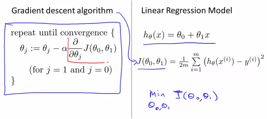
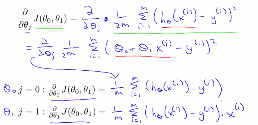
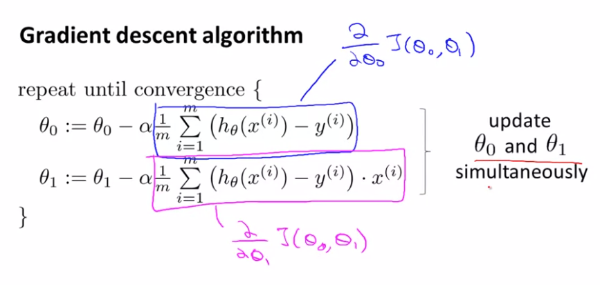
最终的线性回归算法：

进行梯度下降时，可能会得到不同的局部最优解

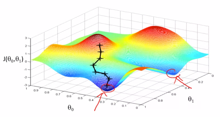
但是事实证明，用于线性回归的代价函数总是一个弓形的函数bowl-shaped（凸函数：Convex function）,这个函数没有任何局部最优解，对这种代价函数使用线性回归只有一个全局最优解。

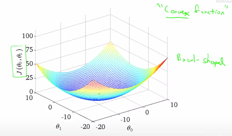
二元参数情形

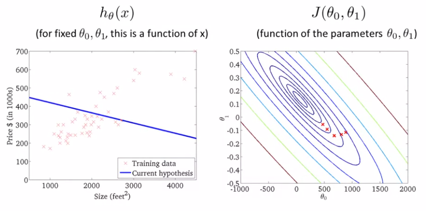
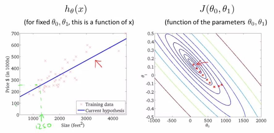
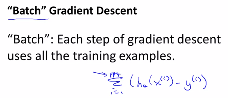
上述的算法也称批量梯度下降，我们在梯度下降的每一步都使用了所有的训练例子，因此梯度下降中计算导数的时候我们计算了m个训练例子的总和。有时梯度下降的其他版本不是成批处理的，他们不是看整个训练集，而是每次去看训练集中的小子集。

求解代价函数J时可以不使用梯度下降这样的迭代法，另一种方法为正规方程法。

阅读材料

Gradient Descent For Linear Regression

When specifically applied to the case of linear regression, a new form of the gradient descent equation can be derived. We can substitute our actual cost function and our actual hypothesis function and modify the equation to :

where m is the size of the training set, \[ \theta_0\] a constant that will be changing simultaneously with \[\theta_1\] and \[x_{i}, y_{i}\] are values of the given training set (data).

Note that we have separated out the two cases for \[ \theta_j\] into separate equations for \[\theta_0\]and \[\theta_1\]; and that for \[\theta_1\] we are multiplying \[ x_{i}\]at the end due to the derivative. The following is a derivation of \[\frac {\partial}{\partial \theta_j}J(\theta)\] for a single example :

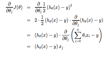
The point of all this is that if we start with a guess for our hypothesis and then repeatedly apply these gradient descent equations, our hypothesis will become more and more accurate.

So, this is simply gradient descent on the original cost function J. This method looks at every example in the entire training set on every step, and is called batch gradient descent. Note that, while gradient descent can be susceptible to local minima in general, the optimization problem we have posed here for linear regression has only one global, and no other local, optima; thus gradient descent always converges (assuming the learning rate α is not too large) to the global minimum. Indeed, J is a convex quadratic function. Here is an example of gradient descent as it is run to minimize a quadratic function.

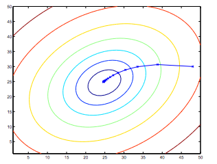
The ellipses shown above are the contours of a quadratic function. Also shown is the trajectory taken by gradient descent, which was initialized at (48,30). The x’s in the figure (joined by straight lines) mark the successive values of θ that gradient descent went through as it converged to its minimum.